Density of States post-processing
Overview of py_dos.py
py_dos.py provides a all-in-one solution to plot and analyze density of states from multiple packages. Here we provides some examples to show its functions.
How to use
The easiest way to use py_dos.py is
- Do a DOS calculation of given package (Like WIEN2K or VASP), keeps all the output files
- Type py_dos.py and press enter
- The DOS is plotted in
dos/plotdos.agr - Use xmgrace dos/plotdos.agr to see the DOS in xmgrace.
- The data are written in
dos/dos.dat.
In general, to quickly view the DOS, just type
$ py_dos.py
$ xmgrace dos/plotdos.agr
We choose SrO as our testing materials. The plot looks like this:
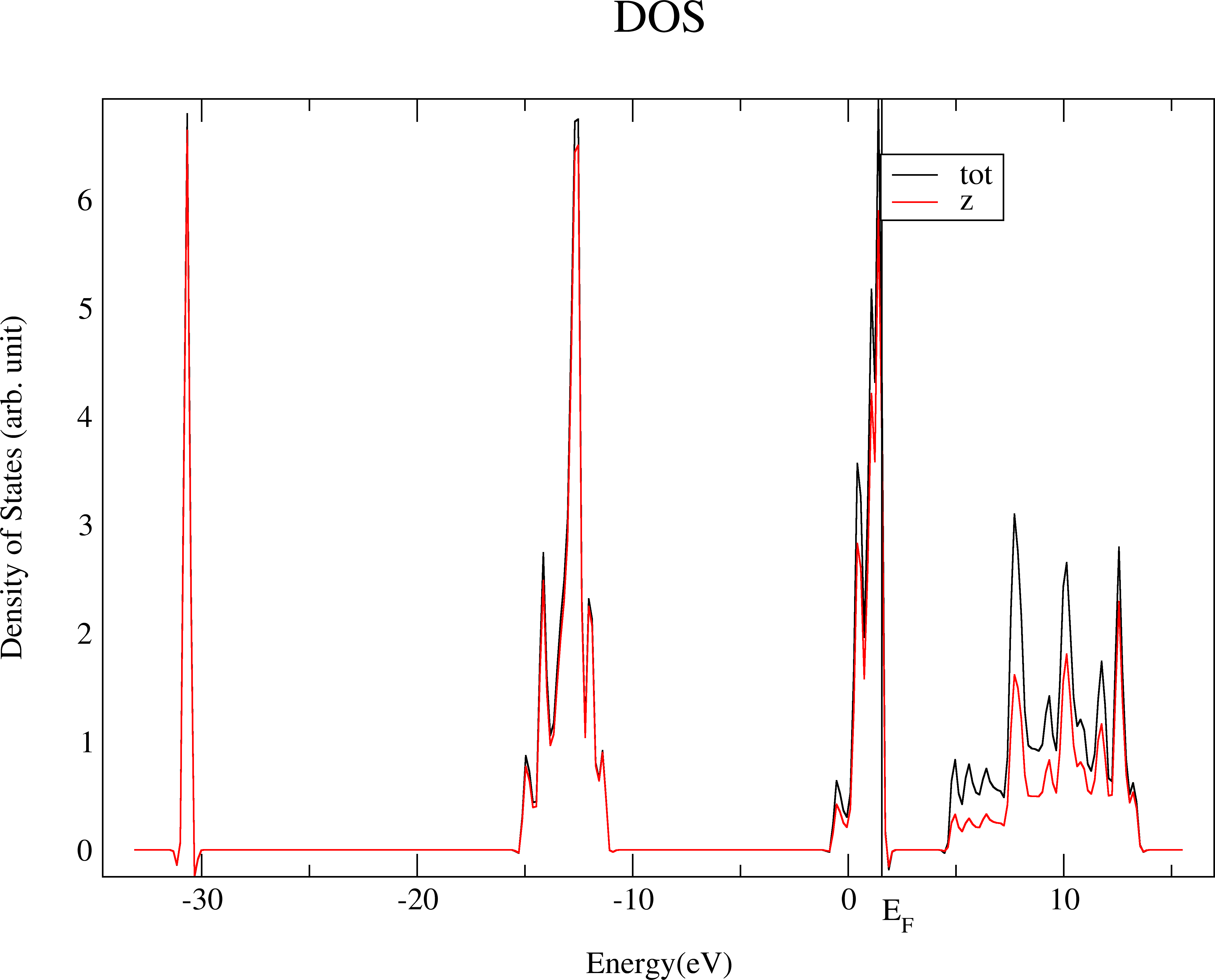
In this picture we can see two lines. The first one is the black line tot and the second one is the red line z. The tot is the total density of states calculated from eigenvalues alone. The z is the summation of all projected density of states. As the projections are not complete, we expects z is always smaller than tot. The difference between these two are larger in the condunction bands because they are more unlocal and not bounded to the atom, or be covererd by atomic projectors.
Better style
The default picture in xmgrace consists of very thin lines if you have never adjust the xmgrace default template.
To make it fit to the paper and slides, we make the lines thicker and characters larger that can be done in xmgrace. After setting all line width to 2 and char size to 1.5, we have
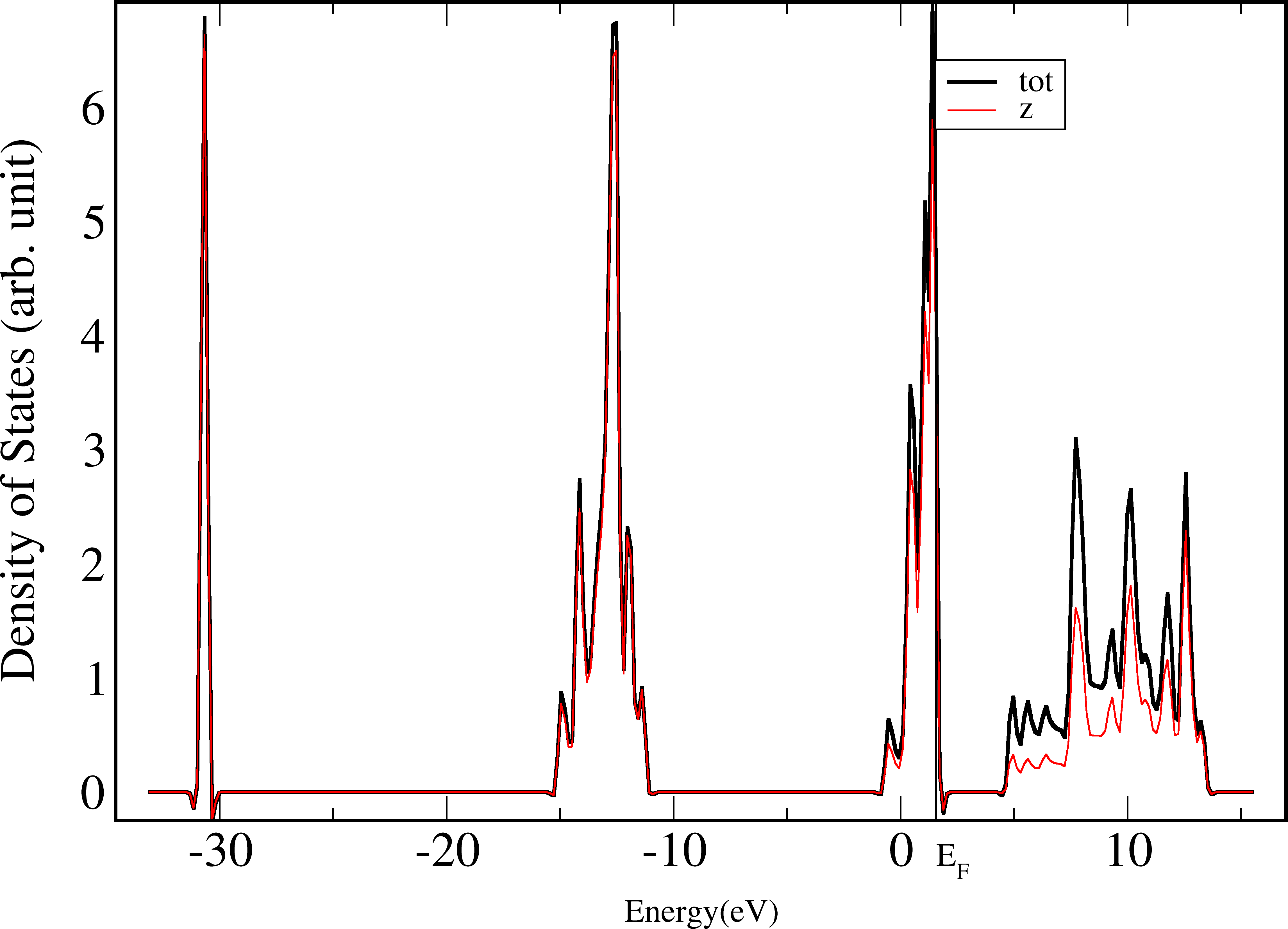
Now this image is much more clear than the default one.
However, we would like to get a .agr file immediately instead of manually modifying it in xmgrace with lots of mouse clicks. It is possible with the option -plotinfo.
$ py_dos.py --plotinfo plotsetting.json
$ xmgrace dos/plotdos.agr
The file plotsetting.json must be created by the user, which can be used multiple times. To achieve the effect above, we define following options:
{"plot_setting":
    {
        "frame linewidth" : 2,
        "line linewidth" : 2,
        "symbol linewidth" : 2,
        "yaxis label char size" : 1.5,
        "yaxis ticklabel char size" : 1.5,
        "xaxis ticklabel char size" : 1.5,
        "title" : "\"\""
    }
}
Align Valence Band Maximum to 0
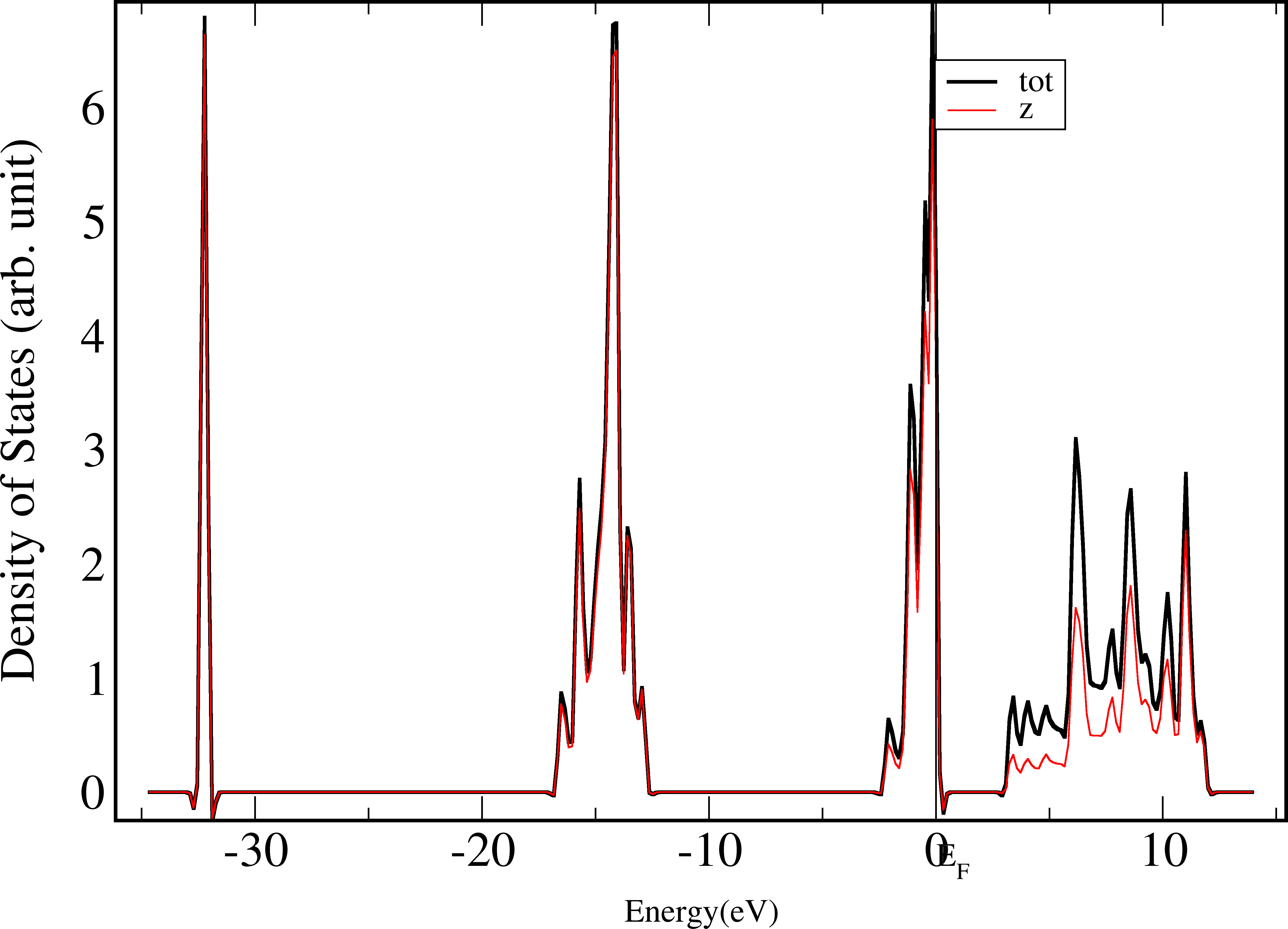
In previous pictures, the valence band maximum (VBM) is indicated as a dashed line (for metals it is the Fermi level), but it is not 0. As plenty of publications use the 0 as the VBM, we can also do it easily here.
$ py_dos.py --plotinfo plotsetting.json -f -g
$ xmgrace dos/plotdos.agr
Where -f means to overwrite the previous dos folder (or you will see nothing changed!) and -g means to put the VBM or Fermi level at 0, and shift all other pictures.
Plot Projected Density of States (PDOS)
In the previous plots, only the total density of states is shown, which does not contains too much information. The PDOS is much more useful in most cases.
In this SrO system, what we concern is the s/p orbitals of Sr and O. To display this PDOS, we use such commands:
$ py_dos.py --plotinfo plotsetting.json -f -g --format "%s(%l)"
$ xmgrace dos/plotdos.agr
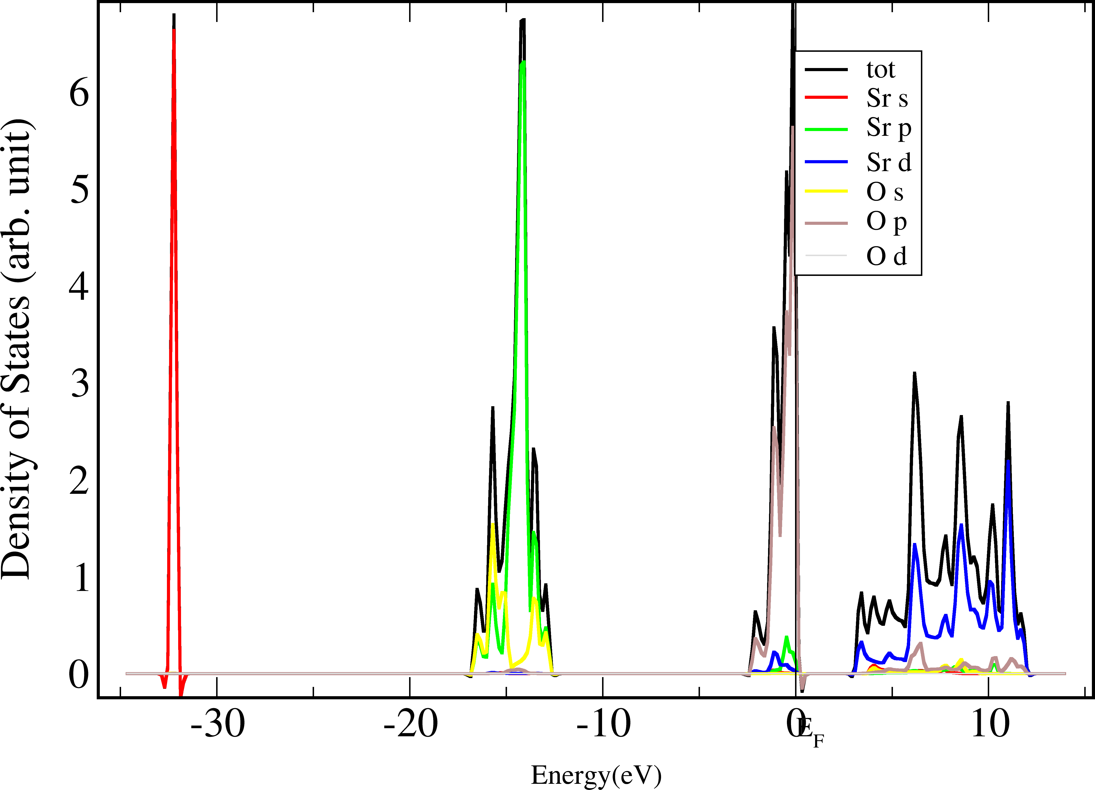
We can see that with just one option -format, all PDOS with Sr(s), Sr(p), Sr(d), O(s), O(p) are plotted and marked. O(p) is the major component of valence bands near Fermi levels, and Sr(d) is the major component of condunction bands. Sr(s) and Sr(p) of inner orbitals are semi-cores and deep below -10eV.
Let us examine how this options works.
The option -format should be followed by an “format string” which indicates what projectors will be plotted. This format string should contains some special marks starting with “%”. Available ones include:
- %s The atom species
- %i The atom index in the whole list
- %n The quantum number n (like 1s/2s/3s orbitals), this is not used in most pseduo-potential packages
- %l The quantum number l (like s/p/d orbitals)
- %m The quantum number m (like px/py/pz orbitals), however different packaged may use different m definition
- %spin The spin (up or down)
This information can uniquely determine where a projetor in any calculations. However, a format string may contains only a few of them, which makes two different projectors looks like the same if we look at only the given marks.
In the plots, py_dos.py take the summation of all the “same” projectors. For example, the format string %s(%l) treats Sr(px), Sr(py), Sr(pz) as the same projector, and plots the summation of them.
Also, the legend name is automatically generated with the format string by directly replacement. If one would like to use legend Sr (orbital s), then we can write the format string like %s (orbital %l).
Filter unwanted PDOS
With the powerful format string, we always plot all PDOS on the picture. Sometimes we do not want some less important orbitals, like O(d). This can be done by filtering those orbitals.
$ py_dos.py -f -g  --format "%s %l" --filter "not (x.species == 'O' and x.l > 1)"   --plotinfo plotsetting_dos.json
$ xmgrace dos/plotdos.agr
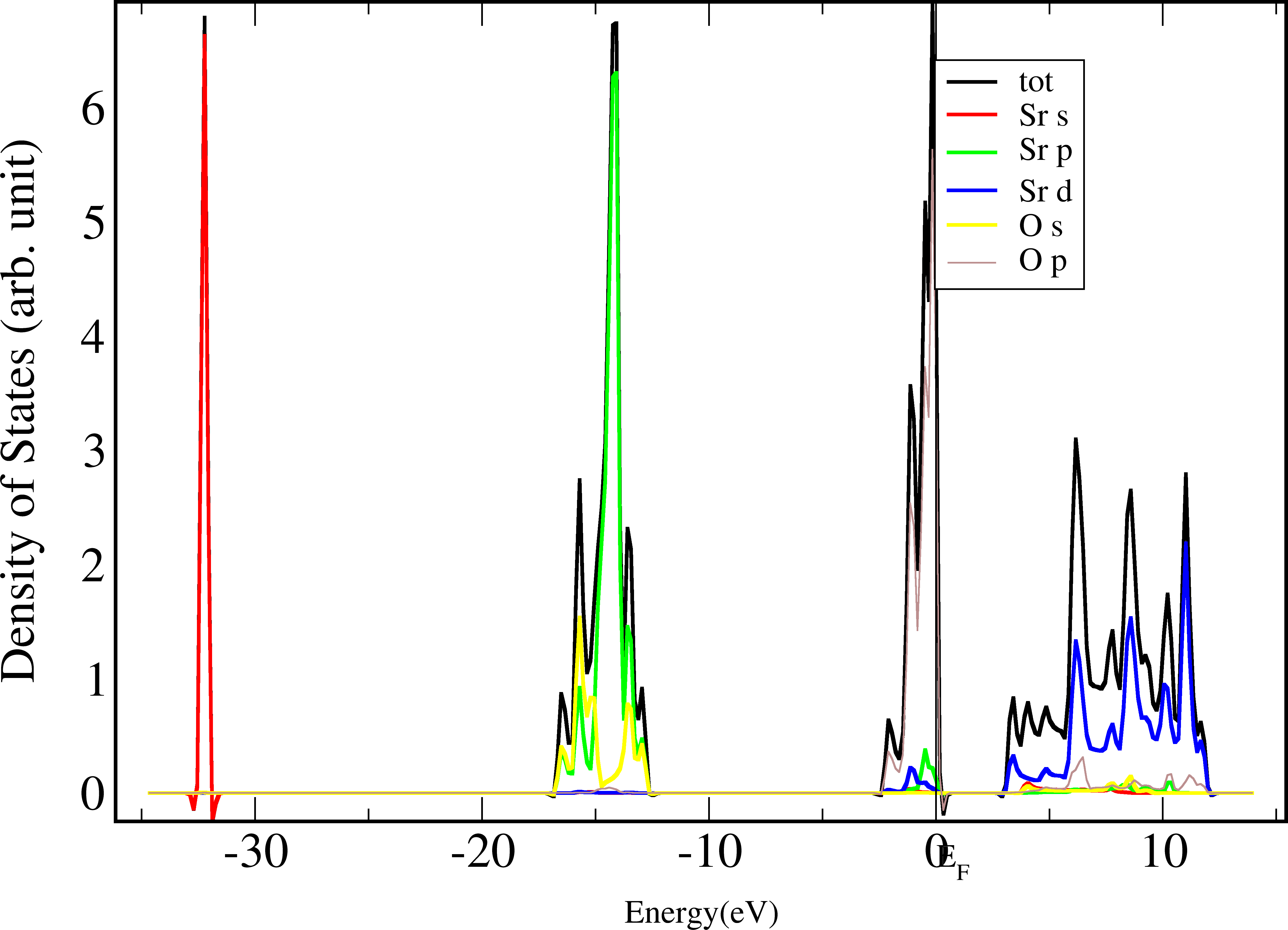
The options filter contains a Python function which returns true or false, only orbitals that returns true will be included in the final plot.
The orbital is represented by an object x in the function. It has propety s, i, n, l, m, spin just the same as the format string. All the options are physical integers, excpet s is an string for element names. spin is -1 or 1 for spin-polarized calculations and 0 for unpolarized calculations.
Here not (x.species == 'O' and x.l > 1) means for all orbitals belongs to oxygen atoms and l quantum numbers larger than 1, or O(d) and O(f), are excluded from the plot.
This function is also useful if you want to see some local DOS, like the first layer of a slab model. The filter then should be like x.i == 1 or x.i == 2 where we assume that the first and the second atoms are the first layer.
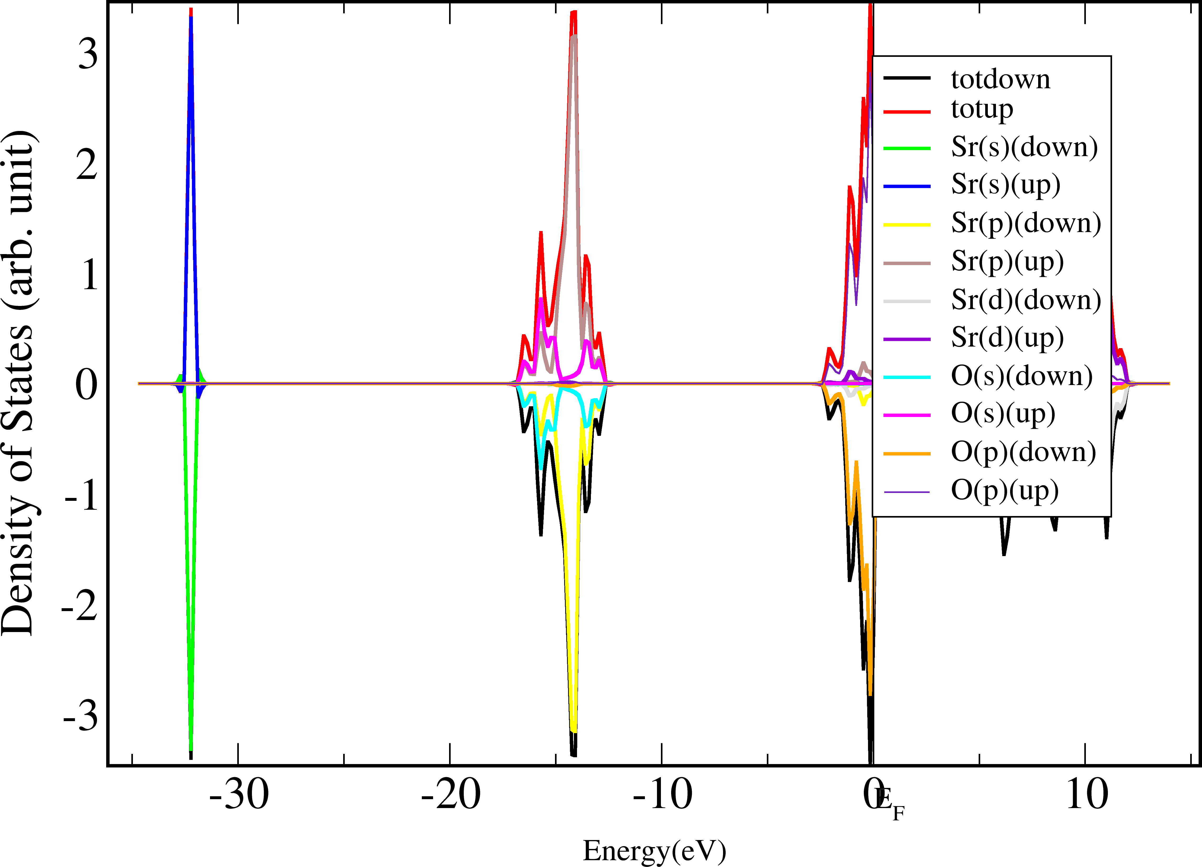
Spin polarized cases
Spin polarized PDOS will be plotted in two sides of the x-axis automatically like
$ py_dos.py  -f -g --format "%s(%l)(%spin)" --filter "not (x.species == 'O' and x.l > 1)"   --plotinfo plotsetting_dos.json
$ xmgrace dos/plotdos.agr
Summary
From above we have already show the what py_dos.py can do.
py_dos.py supports following packages:
- SIESTA : pdos.xml or $CASE$.PDOS
- VASP : none, require to run in the case folder
- WIEN2K : none , require to run in the case folder
- Quantum-Espresso : prefix of output filenames, require to run in the folder contains all output of projwfc.x
Help
The simplified program help file is list below.
usage: py_dos.py [-h] [-i PROGRAM] [-g] [-s] [-d OUTPUTDIR] [-f]
                 [--format FORMAT] [--filter FILTER] [--plotinfo FILEPLOTINFO]
                 [extra_args [extra_args ...]]

Plot DOS of specific package in specific format, also create one-file plain tabular seperated text for DOS.
    File required:
        SIESTA :  pdos.xml or $CASE$.PDOS
        VASP : none, require to run in the case folder
        WIEN2K :  none , require to run in the case folder
        QE :  prefix of output filenames, require to run in the folder contains all output of projwfc.x
    By default, output folder is current folder, so it is sugguested to run this with -d option to redirect output files to another folder as it will create plenty of files.
    Example:
    py_dos.py -d dos --format "%s%i(%l)(%spin)" --filter "x.species=='O'"


positional arguments:
  extra_args            Arguments passed to package-specific procedures

optional arguments:
  -h, --help            show this help message and exit
  -i PROGRAM            The package name
  -g                    Shift band position to make VBM = 0 in graph
  -s                    Do not plot band structure, just write band structure
                        data and k-point list in space-seperated format
  -d OUTPUTDIR          The name of folder used to store output files
  -f                    Control whether to overwrite if the output directory
                        already exists, default is not
  --format FORMAT       Combine multiple DOS into a single one in specific
                        level. Levels include %spin,%m,%l,%n,%i(atom
                        index),%s(species),%t(total). This string also
                        indicates display names, format strings like %x will
                        be replaced while others will be kept
  --filter FILTER       The command to judge whether a specific orbital should
                        be included in final results, like 'x.l ==1 and x.i <
                        70'. Warning: This string will be EXECCUTED DIRECTLY
                        so be cautious!
  --plotinfo FILEPLOTINFO
                        The input file for plotting parameters